
ルンゲ=クッタ法
ルンゲ=クッタ法(runge kutta method)は微分方程式を数値的に解く手法の一つで、そのプログラムの実装の容易さから時間発展追跡の簡便法として知られています。特に4次のルンゲ=クッタ法(RK4法)は計算コストと計算精度の兼ね合いから広く用いられています。RK4法は時刻 $t$ の関数 $x = x(t)$ の常微分方程式
\dfrac{dx}{dt}=f(x,t) \tag{1}
について、以下の式を用いて時間 $\Delta t$ だけ進んだときの方程式$(1)$の解 $x=x(t+\Delta t)$ を求めます。
x_{n+1}=x_n+\frac{\Delta t}{6} k_1+\frac{\Delta t}{3} k_2+\frac{\Delta t}{3} k_3+\frac{\Delta t}{6} k_4 \tag{2}
ここで、$k_1$~$k_4$は以下の式で与えられます。
\begin{cases}
k_1 =f\left(x_n,\, t_n\right)\\
k_2 =f\left(x_n+\dfrac{\Delta t}{2} k_1,\, t_n+\dfrac{\Delta t}{2}\right) \\
k_3 =f\left(x_n+\dfrac{\Delta t}{2} k_2,\, t_n+\dfrac{\Delta t}{2}\right) \\
k_4 =f\left(x_n+\Delta t \, k_3,\, t_n+\Delta t\right)
\end{cases} \tag{3}
この操作を繰り返すことで時間発展を追跡することができます。
化学反応の速度論
遷移状態理論の範囲では、反応速度定数はアイリングの式に基づいて温度$T$と活性化エネルギー$\Delta G^{\ddagger}$をパラメータとして与えられます。
k=\varGamma \dfrac{k_{\mathrm{B}}T}{h} \, \exp \left(-{\dfrac{\Delta G^{\ddagger}}{RT}}\right)
ここで$\varGamma$は透過係数を表し、トンネル効果の補正を考慮しない場合は $\varGamma=1$ として計算するのが通例です。
A、B、Cの3状態からなる1次の逐次反応モデルを考えます。正反応(forward reaction)には "f"、逆反応(reverse reaction)には "r" とラベリングしています。
\large [\mathrm{A}] \underset{k_{1r}}{\overset{k_{1f}}{\rightleftarrows}} [\mathrm{B}] \underset{k_{2r}}{\overset{k_{2f}}{\rightleftarrows}} [\mathrm{C}]
この系が、例えば以下のようなエネルギーダイアグラム(縦軸は自由エネルギー)で表現される場合を考えます。
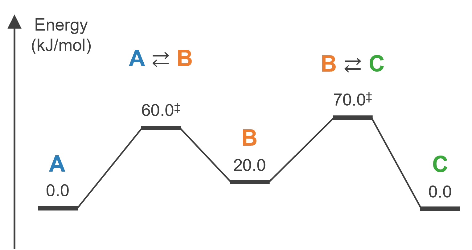
このとき反応速度定数は 300 K において、それぞれ次のようになります。
k1f = 2.234724e+02
k1r = 6.783680e+05
k2f = 1.231245e+04
k2r = 4.056047e+00
これらの値の計算方法については以下の記事を参考にしてください。
https://qiita.com/h-nabata/items/ada3098b933e17613dca
したがって、この系のレート方程式は 300 K において以下のようになります。
\begin{aligned}
\dfrac{d[\mathrm{A}]}{dt} &= − 2.23 \times 10^{2} [\mathrm{A}] + 6.78 \times 10^{5} [\mathrm{B}] \\
\dfrac{d[\mathrm{B}]}{dt} &= 2.23 \times 10^2 [\mathrm{A}] − 6.78 \times 10^5 [\mathrm{B}] − 1.23 \times 10^4 [\mathrm{B}] + 4.05 \times 10^0 [\mathrm{C}] \\
\dfrac{d[\mathrm{C}]}{dt} &= 1.23 \times 10^4 [\mathrm{B}] − 4.05 \times 10^0 [\mathrm{C}]
\end{aligned}
この連立微分方程式をPythonのコードに起こすと次のような関数として表現できます。関数 reaction_equations() の引数は次の通り。
- 各状態の濃度
concentrations(floatのlist)
def reaction_equations(concentrations):
    # Define the system of ordinary differential equations
    # Modify this function according to your specific reaction system
    A, B, C = concentrations
    dAdt = - k1f * A + k1r * B
    dBdt = k1f * A - k1r * B - k2f * B + k2r * C
    dCdt = k2f * B - k2r * C
    return [dAdt, dBdt, dCdt]
これにRK4法を適用していきます。
RK4法による速度論シミュレーション
RK4法をPythonのコードに起こすと次のような関数として表現できます。関数 runge_kutta() の引数は次の通り。
- 時間の刻み幅
dt(float) - シミュレーション時間の最大値
t_max(float) - 初期濃度
initial_concentrations(floatのlist)
def runge_kutta(dt, t_max, initial_concentrations):
    # Perform the simulation using the fourth-order Runge-Kutta method
    t = 0.0
    concentrations = np.array(initial_concentrations)
    time_points = [t]
    concentration_points = [concentrations]

    while t < t_max:
        # Compute concentration changes using the fourth-order Runge-Kutta method
        k1 = reaction_equations(concentrations)
        k2 = reaction_equations(concentrations + 0.5 * dt * np.array(k1))
        k3 = reaction_equations(concentrations + 0.5 * dt * np.array(k2))
        k4 = reaction_equations(concentrations + dt * np.array(k3))
        concentrations += (dt / 6.0) * (np.array(k1) + 2 * np.array(k2) + 2 * np.array(k3) + np.array(k4))
        t += dt

        time_points.append(t)
        concentration_points.append(concentrations.copy())

    return time_points, np.array(concentration_points)
あとはこれらのコードを組み合わせるだけです。ついでに各濃度の時間発展の推移も描画してみましょう。スクリプト全体は次のようになります。
import numpy as np
import matplotlib.pyplot as plt
import sys

k1f = 2.234724e+02
k1r = 6.783680e+05
k2f = 1.231245e+04
k2r = 4.056047e+00

def reaction_equations(concentrations):
    # Define the system of ordinary differential equations
    # Modify this function according to your specific reaction system
    A, B, C = concentrations
    dAdt = - k1f * A + k1r * B
    dBdt = k1f * A - k1r * B - k2f * B + k2r * C
    dCdt = k2f * B - k2r * C
    return [dAdt, dBdt, dCdt]

def runge_kutta(dt, t_max, initial_concentrations):
    # Perform the simulation using the fourth-order Runge-Kutta method
    t = 0.0
    concentrations = np.array(initial_concentrations)
    time_points = [t]
    concentration_points = [concentrations]

    while t < t_max:
        # Compute concentration changes using the fourth-order Runge-Kutta method
        k1 = reaction_equations(concentrations)
        k2 = reaction_equations(concentrations + 0.5 * dt * np.array(k1))
        k3 = reaction_equations(concentrations + 0.5 * dt * np.array(k2))
        k4 = reaction_equations(concentrations + dt * np.array(k3))
        concentrations += (dt / 6.0) * (np.array(k1) + 2 * np.array(k2) + 2 * np.array(k3) + np.array(k4))
        t += dt

        time_points.append(t)
        concentration_points.append(concentrations.copy())

    return time_points, np.array(concentration_points)

# Example usage
dt = 1e-6  # Time step size
t_max = 1e+0  # Maximum simulation time
initial_concentrations = [1.0, 0.0, 0.0]  # Initial concentrations of species A, B, C
time_points, concentration_points = runge_kutta(dt, t_max, initial_concentrations)
print(concentration_points[-1])  # showing the result

# Plotting the concentration curves
plt.plot(time_points[1:], concentration_points[1:, 0], label='A')
plt.plot(time_points[1:], concentration_points[1:, 1], label='B')
plt.plot(time_points[1:], concentration_points[1:, 2], label='C')
plt.xlabel('Time')
plt.ylabel('Concentration')
plt.legend()
plt.show()
[5.00091038e-01 1.64741207e-04 4.99744221e-01]
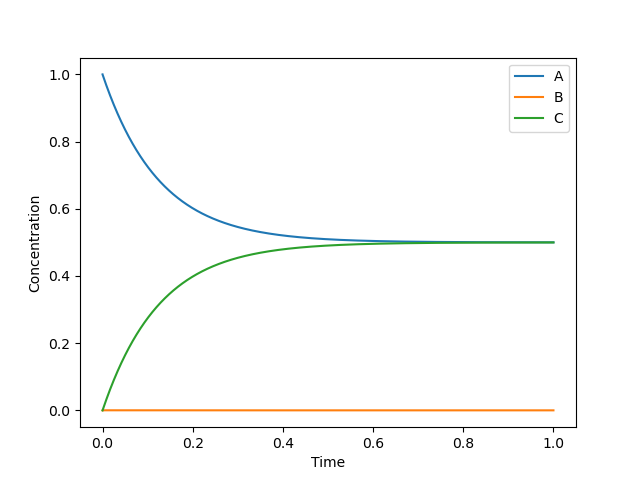
この系では1秒後までに完全に熱平衡に達することが分かります。
Stiff問題
最後に、化学反応の速度論解析における問題点について紹介しておきます。
解析学の分野では「Stiff問題」というシミュレーション上の問題が知られています。"stiff" は「固い」を意味する語で、係数のオーダーが極めて広い範囲にわたる微分方程式を数値的にシミュレーションする際に浮上する問題の原因が、方程式の "stiffness"(固さ)です。
化学反応の場合、メチル基の内部回転のような速い素過程(~$10^{-12}$秒に1回程度)と結合の組み換えのような遅い素過程(~$10^{3}$秒に1回程度)が混在しており、微分方程式の係数のレンジが$10^{15}$オーダーに亘ることがしばしばあります。
このような場合、刻み幅 $\Delta t$ を大きくすると数値解が不安定化し、速い素過程による数値誤差の蓄積(=発散)が生じることが知られています。そのため刻み幅 $\Delta t$ は十分小さくする必要がありますが、そうすると今度は計算時間が増大するため長時間のシミュレーションが難しくなってしまいます。
解析学の分野ではこのような問題を「Stiff問題」と呼んでいます。実際に化学反応の濃度変化をシミュレーションしてみるとよく分かりますが、速度論シミュレーションにおいてstiff問題は頻繁に出現します。これを回避する速度論解析手法として「反応速度定数行列縮約法」などが知られています。この手法について本稿では詳しく立ち入りませんので、興味のある方は参考文献を参照してください。
参考文献
- RK4法で用いる$k_1$~$k_4$の図形的な意味を解説した動画:
https://www.youtube.com/watch?v=1YZnic1Ug9g
- 反応速度定数行列縮約法について:
https://www.jstage.jst.go.jp/article/mssj/21/2/21_151/_article/-char/ja/