igraphについて　

グラフの作成・操作を行うライブラリ（内部はC/C++系）。2023年2月現在の最新バージョンは 0.10.4 。
【参考】公式サイト

RやPythonで利用可能なigraphパッケージが公開されている。今回はPython版を利用する。

pip install igraph または conda install -c conda-forge python-igraph によりインストール可能（公式ドキュメント）。

かつてはPyPIにおいて "igraph" と "python-igraph" という2つのパッケージが競合してしまい、pipでは正しくインストールできないという問題が生じていたが、現在では解消されている。

ネットワークの生成

以下のようなスクリプトにより、グラフの頂点の数、辺の数とそれによって接続される節点を指定してネットワークを作成できる。

スクリプト①

import matplotlib.pyplot as plt
import igraph

fig, ax = plt.subplots()

g = igraph.Graph()
g.add_vertices(3)
g.add_edges([(0,1), (1,2)])

print(g)

my_layout = g.layout_auto()
igraph.plot(g, layout = my_layout, target= ax)
plt.show()

実行結果は以下。

出力①

IGRAPH U--- 3 2 --
+ edges:
0--1 1--2

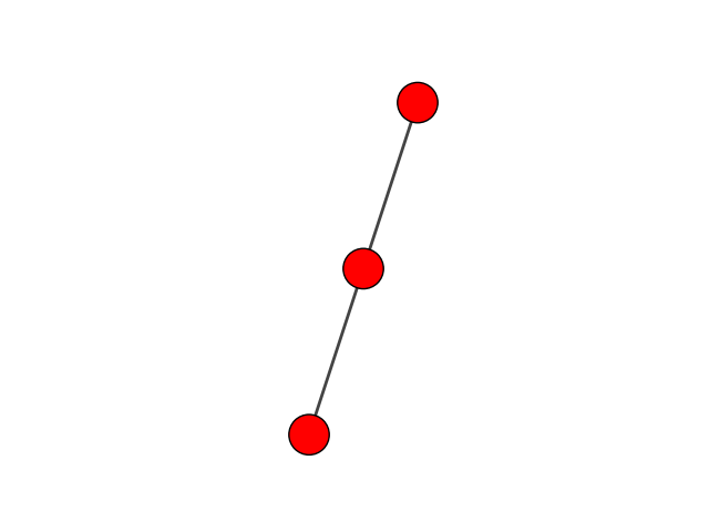
ネットワークそのものは、このようにして生成することができる。なお、printの代わりにsummaryとするとエッジの出力が省略される。大規模グラフの確認の際にはsummaryを使うのがよい。

頂点、辺、節点の追加

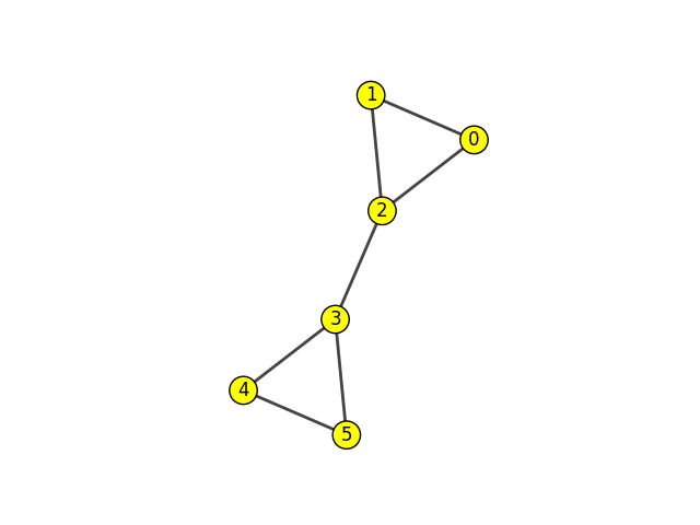
これに対して、さらに頂点、辺、節点を増やすことができる。

スクリプト②

import matplotlib.pyplot as plt
import igraph

fig, ax = plt.subplots()

g = igraph.Graph()
g.add_vertices(3)
g.add_edges([(0,1), (1,2)])

# added
g.add_edges([(2, 0)])
g.add_vertices(3)
g.add_edges([(2, 3), (3, 4), (4, 5), (5, 3)])

print(g)

# specifing the plot style
visual_style ={
    "vertex_color": "yellow",
    "vertex_size":0.2,
    "vertex_label":[0,1,2,3,4,5]
}

my_layout = g.layout_auto()
igraph.plot(g, layout = my_layout, target= ax, **visual_style)
plt.show()

出力②

IGRAPH U--- 6 7 --
+ edges:
0--1 1--2 0--2 2--3 3--4 4--5 3--5

頂点、辺、節点の削除

ここで、上記スクリプト②において、例えば g.delete_edges(3) という行を末尾に追加すると、2--3 の辺が消える。
複数の辺を消去するには g.delete_edges([(0,2),(2,3),(3,4)]) のように指定すればよい。

スクリプト③

import matplotlib.pyplot as plt
import igraph

fig, ax = plt.subplots()

g = igraph.Graph()
g.add_vertices(3)
g.add_edges([(0,1), (1,2)])

g.add_edges([(2, 0)])
g.add_vertices(3)
g.add_edges([(2, 3), (3, 4), (4, 5), (5, 3)])

print(g)

visual_style ={
    "vertex_color": "yellow",
    "vertex_size":0.2,
    "vertex_label":[0,1,2,3,4,5]
}

# added
g.delete_edges([(0,2),(2,3),(3,4)])

my_layout = g.layout_auto()
igraph.plot(g, layout = my_layout, target= ax, **visual_style)
plt.show()

出力③

IGRAPH U--- 6 7 --
+ edges:
0--1 1--2 0--2 2--3 3--4 4--5 3--5

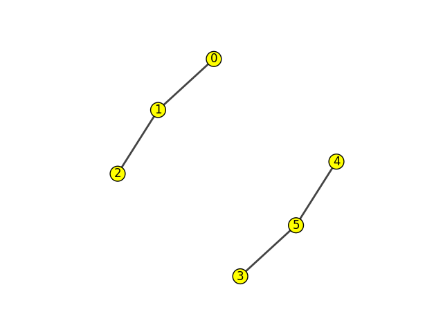
0--2、2--3、3--4 の3辺が切断されたことが分かる。

ネットワークを確率的に生成する

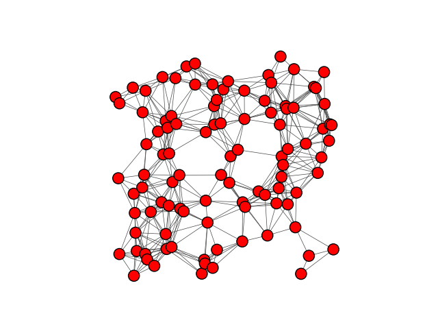
Graph.GRG(頂点数、距離の閾値) によって、指定された頂点数を有するグラフを確率的に生成することができる。

スクリプト④

import matplotlib.pyplot as plt
import igraph

fig, ax = plt.subplots()

g = igraph.Graph()
g = igraph.Graph.GRG(100, 0.2)

igraph.summary(g)

visual_style ={
    "vertex_size":0.05,
    "edge_width":0.5
}

my_layout = g.layout_auto()
igraph.plot(g, layout = my_layout, target= ax, **visual_style)
plt.show()

出力④

IGRAPH U--- 100 517 --
+ attr: x (v), y (v)

ネットワークをツリー状に生成する

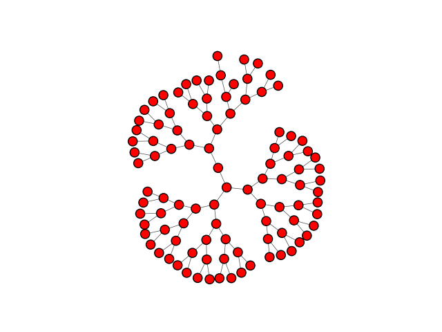
Graph.Tree(頂点数、木の分岐数) によって、指定された頂点数および分岐数の木構造を有するグラフを生成することができる。

スクリプト⑤

import matplotlib.pyplot as plt
import igraph

print(igraph.__version__)

fig, ax = plt.subplots()

g = igraph.Graph()
g = igraph.Graph.Tree(100, 2)

igraph.summary(g)

visual_style ={
    "vertex_size":0.5,
    "edge_width":0.5
}

my_layout = g.layout_auto()
igraph.plot(g, layout = my_layout, target= ax, **visual_style)
plt.show()

出力⑤

IGRAPH U--- 100 99 --

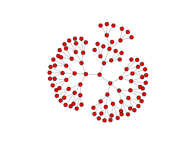
また、g = igraph.Graph.Tree(100, 3) とすると、以下のような三又に分岐したグラフが得られる。

有向グラフの生成

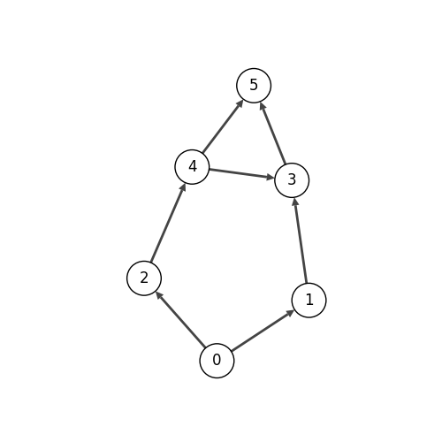
有向非巡回グラフ(Directed Acyclic Graph: DAG)の場合、以下のようにしてトポロジカルソートを取得することができる。igraph.Vertex.indegree() によって各ノードの次数を求めることができる。

「有向非巡回グラフ」とは、閉路のない有向グラフのこと。ある頂点から有向線分の向きに辺を辿るとき、同じ頂点に戻れないという特徴がある。

スクリプト⑥

import matplotlib.pyplot as plt
import igraph

g = igraph.Graph(
    edges=[(0, 1), (0, 2), (1, 3), (2, 4), (4, 3), (3, 5), (4, 5)],
    directed=True,
)

assert g.is_dag
results = g.topological_sorting(mode='out')
print('Topological sort of g (out):', *results)

for i in range(g.vcount()):
    print('degree of {}: {}'.format(i, g.vs[i].indegree()))

fig, ax = plt.subplots(figsize=(5, 5))
igraph.plot(
        g,
        target=ax,
        vertex_size=0.4,
        edge_width=2,
        vertex_label=range(g.vcount()),
        vertex_color="white",
    )

plt.show()

ここで、edgesを定義する際に (0, 1), (1, 0) などのように、同じノードの組に対して逆向きの2辺を指定することはできないので注意。

出力⑥

Topological sort of g (out): 0 1 2 4 3 5
degree of 0: 0
degree of 1: 1
degree of 2: 1
degree of 3: 2
degree of 4: 1
degree of 5: 2

参考：有向非巡回グラフ（DAG）とトポロジカルソート

重み付きグラフの生成

igraphを用いて、各辺が重み付けされたグラフを解析することができる。重み付きグラフで最短経路を取得する場合、 g.get_shortest_paths() 関数の引数として、各辺の重み weights=g.es["weight"] と出力方法 output="epath" を渡す。

スクリプト⑦

import matplotlib.pyplot as plt
import igraph


g = igraph.Graph(
    8,
    [(0, 1), (0, 2), (1, 3), (1, 7), (2, 3), (2, 4), (3, 5), (3, 7), (4, 5), (4, 6), (4, 7), (6, 7)]
)

# adding weights to the edges
g.es["weight"] = [2, 1, 5, 4, 6, 3, 2, 1, 4, 2, 2, 4]

results = g.get_shortest_paths(0, to=5, weights=g.es["weight"], output="epath")
print(*results)

if len(results[0]) > 0:
    # Add up the weights across all edges on the shortest path
    distance = 0
    for e in results[0]:
        distance += g.es[e]["weight"]
    print("Shortest weighted distance is: ", distance)
else:
    print("End node could not be reached!")

g.es['width'] = 1.0
g.es[results[0]]['width'] = 2.5

fig, ax = plt.subplots()
igraph.plot(
    g,
    target=ax,
    layout='circle',
    vertex_color='steelblue',
    vertex_label=range(g.vcount()),
    edge_width=g.es['width'],
    edge_label=g.es["weight"],
    edge_color='#666',
    edge_align_label=True,
    edge_background='white'
)

plt.show()

出力⑦

[1, 5, 8]
Shortest weighted distance is:  8

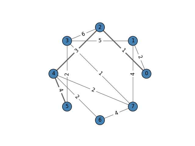
ノード0からノード5に至る経路のうち、総コストが最小となる経路が正しく得られている。

参考資料

https://qiita.com/scapegoat_11_/items/d99cbcfea053d9fcd8d2

↓ 公式ドキュメントにあるグラフの見本、サンプルコード

https://igraph.readthedocs.io/en/stable/tutorials/index.html

https://igraph.readthedocs.io/en/stable/tutorials/topological_sort.html

https://igraph.readthedocs.io/en/stable/tutorials/shortest_path_visualisation.html

Qiita Articles

【Python】igraphでグラフ・ネットワークを生成・描画する